The traveling salesman problem

One question of particular interest is how to route emergency aid to locations where it is needed. For concreteness, let’s postulate a Red Cross medical or food supply caravan that originates from the organization’s in-country headquarters. This caravan wishes to visit all $n$ emergent locations in order to deliver needed supplies. They wish to do so in the most efficient manner possible.

This is the traveling salesman problem (TSP), an optimization problem that is quite well known. It was first described in 1932 by Karl Menger and has been studied extensively ever since. Here is the traditional convex optimization specification of the problem:

$$\begin{aligned} \min &\sum_{i=0}^n \sum_{j\ne i,j=0}^nc_{ij}x_{ij} && \\ \mathrm{s.t.} & \\ & x_{ij} \in \{0, 1\} && i,j=0, \cdots, n \\ & \sum_{i=0,i\ne j}^n x_{ij} = 1 && j=0, \cdots, n \\ & \sum_{j=0,j\ne i}^n x_{ij} = 1 && i=0, \cdots, n \\ &u_i-u_j +nx_{ij} \le n-1 && 1 \le i \ne j \le n\end{aligned}$$

As is clear from the constraints, this is an integer linear program (ILP) where:

• $x_{ij}$ is a binary decision variable indicating whether we go from location $i$ to location $j$.
• $c_{ij}$ is the distance between location $i$ and location $j$. (Note: in our application, we deal with geospatial data on a large enough scale that the Euclidean distance is actually very imprecise. In order to model distances over the planet’s surface, we use the Haversine formula.)
• The objective function is the sum of the distances for routes that we decide to take.
• The final constraint ensures that all locations are visited once and only once.

The problem, of course, is that brute force solution of the TSP is $\mathcal{O}$$(n!)$. Traditional, deterministic algorithm approaches such as branch-and-bound or branch-and-cut are still impractical for larger numbers of nodes. In many cases, exhaustive search for global optimality is not even particularly helpful as long as the solution found is good enough. We will use simulated annealing (SA) to get acceptable solutions to the TSP.

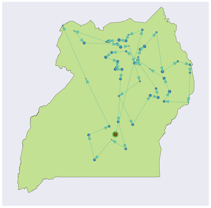
Figure 8 shows a sample draw of conflict data (the blue points), and a near-optimal TSP route found through 50,000 iterations of simulated annealing.

Packing the aid truck — the Knapsack Problem

We extend the TSP into a multi-objective optimization problem where the contents of the aid trucks also have an optimization component. Therein lies the knapsack problem: subject to a volume or weight constraint, and given that different locations might have very different needs such as food, vaccinations, or emergent medical supplies, which supplies do we pack on the trucks?

Often, this problem is formulated such that you can only bring one of each item, but that does not make sense in our application. Rather, we want to be able to bring as many types of each type of aid as we think necessary, and we’ll assume that as many as desired are available to load on the trucks before starting out from HQ. Here’s the unbounded version of the knapsack problem:

$$\begin{aligned} \max &\sum_{i=1}^n v_i x_i && \\ \mathrm{s.t.} & \\ & x_i \in \mathbb{Z} \\ & x_i \geq 0 \\ & \sum_{i=1}^n w_ix_i \leq W\end{aligned}$$

In this formulation:

• $x_{i}$ is a zero or positive integer decision variable indicating how many units of item $i$ we load on the truck.
• $v_i$ is the utility we get from bringing along item $i$.
• $w_i$ is the weight of item $i$.
• $W$ is the maximum weight the truck can carry.

A brief detour for modeling assumptions

Before we can optimize this aid delivery mechanism, we will need to decide a way to model humanitarian aid needs at a given conflict.

Let us assume that there are $K$ distinct types of humanitarian aid to be delivered. (Without loss of generality, we will use three categories for all of our examples — perhaps we can think of them food aid, first aid supplies, and medicines for concreteness.) We can model each conflict’s aid needs as

$$\boldsymbol x \sim \mathrm{Dir}(\boldsymbol \alpha)$$

where $\boldsymbol \alpha$ parameterizes the distribution to generate vectors of length $K$ representing the relative proportions of needs. For example, in our three category example we might draw the vector $(0.11,\,0.66,\,0.23)$ for a certain conflict, meaning that 11% of the aid needed at this conflict is food aid, 66% is first aid supplies, and 23% is medicines. Now that we know the proportions for the given conflict, how might we turn this unitless vector into absolute amounts?

For that reason, let’s assign each conflict a scaled size $s \in [1, 10]$ based on the number of casualties (a proxy for the severity of the conflict). We can use this size scalar to turn our proportion vector into a vector of absolute needs.

It should be noted that both of these modeling methods for proportions and size are “plug-and-play” — because of purposely designed loose coupling in our model, these methods could trivially be replaced by a different method of calculating or predicting the needs of each conflict. For example, if an independent model was used to calculate each of $K$ needs based on the features of each conflict, those quantities could easily be plugged in to this model. Ultimately, the only quantities that our TSP/Knapsack model needs is an $n \times K$ matrix of aid needs for $n$ cities and $K$ categories of aid.

A new objective function to integrate TSP and Knapsack

For the vanilla TSP, we simply try to minimize the total distance. Now that we are adding a new objective, we will need to integrate the two into a coherent loss function. Here is the function we will actually try to minimize in the combined TSP/Knapsack:

$$L(\boldsymbol x) = \text{total distance} + \text{sum of squared aid shortfalls}$$

The effect of squaring aid shortfalls acts as a weight, causing greater importance to be placed on minimizing this aspect of the problem first. Proposals wherein aid shortfalls occur are heavily penalized. As we will see in later graphs, once the SA algorithm is able to avoid all shortfalls and the concurrent massive loss function penalties, a much slower descent begins to take place wherein the distance is slowly optimized. See figure 10 for a depiction of this phenomenon.

Implementing the Knapsack aspect

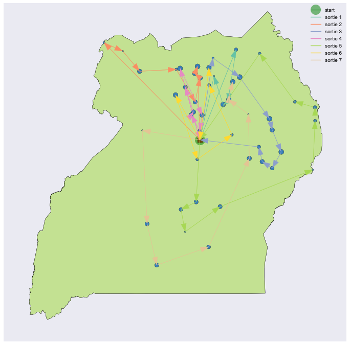
Figure 9 shows the same draw of cities as in figure 8, this time factoring in limited carrying capacity for aid supplies on the aid delivery mechanism and using our new loss function. As we can see, the huge penalty incurred when supplies run out quickly induces the simulated annealing algorithm to converge on a solution with multiple stops at HQ to reload.

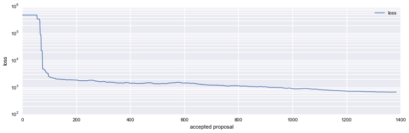
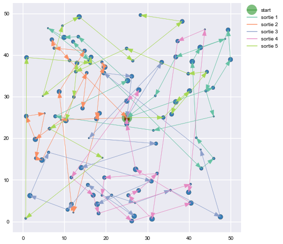
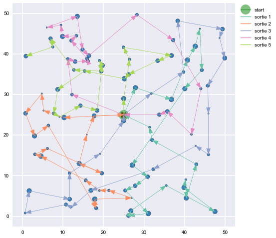
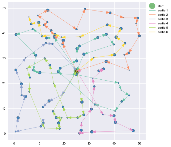
Figures 11, 12, and 13 use some uniformly distributed points on the $[0,50]$ plane to demonstrate how the proposed TSP/Knapsack routes converge as the number of iterations increases.

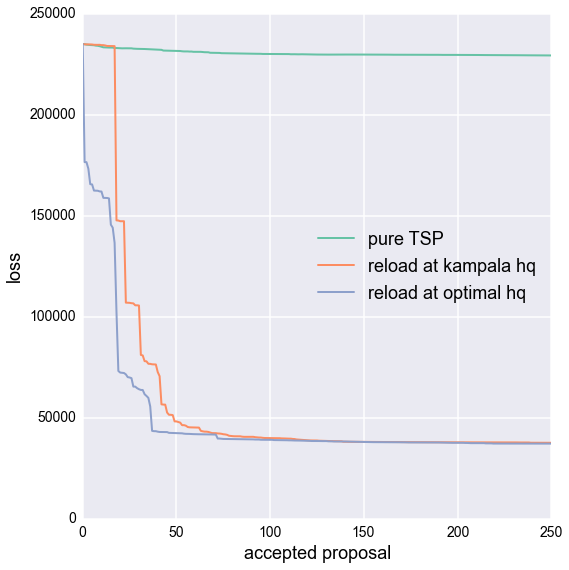
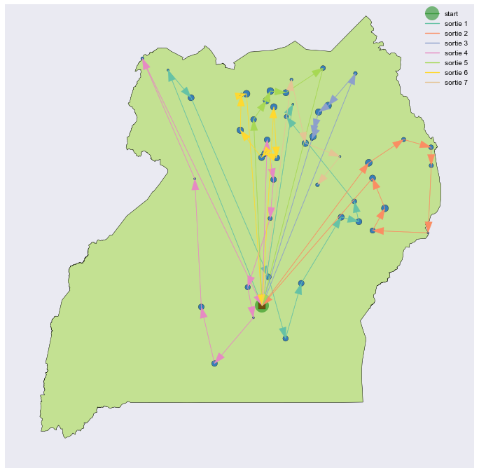
Finding the optimal site for the resupply location

Our initial assumption was that the HQ was located in the capital city of Kampala. However, we should ask whether our HQ could be more conveniently located. We can answer this question by treating the reload location as another parameter and continuing to sample HQ locations using SA. Figure 14 shows the TSP/Knapsack optimized once again, this time using a the optimal HQ location, while figure 15 compares the loss function as each method converges to its best possible configuration.