Events in space

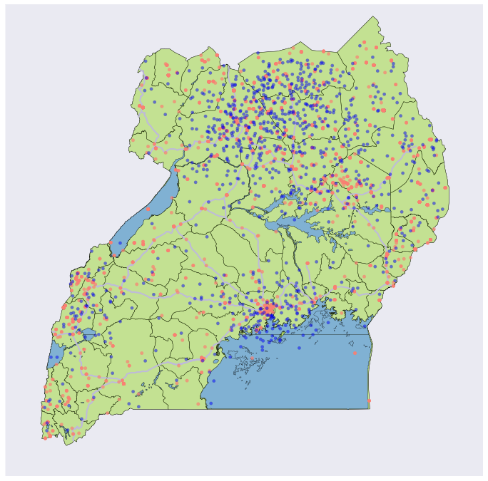
The violence and civil conflict events described in the ACLED dataset are coded with both a latitude and a longitude. One assumption we make is that these events are distributed due to underlying causes such as population centers, road access, historical land ownership, and other features that make conflicts more or less likely. It is difficult to directly create a generative model for these probabilities, so we will make the further assumption that the distribution of the data already incorporates and is representative of these factors. In effect, we treat the entire country of Uganda as a probability distribution from which geospatial conflict events could be sampled. We took historical conflict location data from the entire ACLED data set and smoothed it using a Matérn covariance function. Figure 2 shows this smoothing applied to the same conflicts depicted in figure 1.

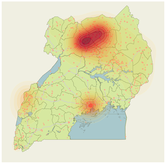
We used this smooth function as a kernel-density esitmate (KDE). This estimate (i.e., the empirical distribution of the conflict data), has a complex functional form which makes it challenging to sample from. However, for any given coordinate it is quite simple to get the probability of an event. Given this property of our KDE, we can apply Monte Carlo sampling techniques to generate samples from this probability distribution. Visualizing the distribution, we can see that it is multi-modal with regions of low density between the modes. Because of these properties, we opted to use slice sampling to generate draws from the distribution.

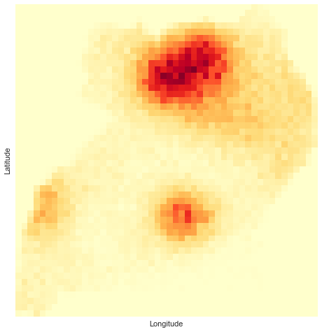
Figure 3 shows the first 1,000 samples from this probability distribution. (Note: we throw away samples that occur over water or outside of country boundaries.) Figure 4 shows the distribution of the samples as a two-dimensional histogram.

 

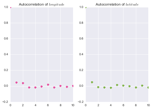
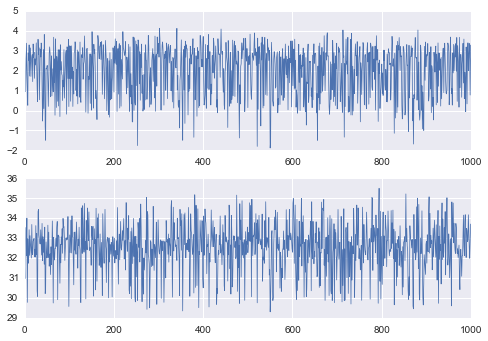
When slice sampling, there are a number of parameter choices that are imporant. We want to choose our rectangle widths, burn-in, and thinning parameters appropriately. In testing, a thinning value of 10 reduced autocorrelation to less than 0.1 at a time lag of 1. We can see this result in figure 5. We used the Gelman-Rubin potential scale reduction factor to determine if we were observing favorable mixing. Generally, a value less than 1.1 indicates good mixing. In both of our dimensions, the Gelman-Rubin statistic was less than this threshold. We also calculated the Geweke statistic, which is used to indicate convergence. A value less than 2 indicates convergence and for our draws, this statistic was $\ll$ 1. We can also examine convergence by looking at the trace plots for the samples. As we see in figure 6 these appear stationary.

Events in time

As a modeling assumption, we separate the dimensions of space and time as being independent. To model events in time across the country, we use an autoregressive Poisson GLM. While standard autoregressive models create a linear relation between a future value and a previous value, the Poisson GLM permits a linear relation between previous data and the mean of a Poisson distribution. This will allow us to retain the probabilistic interpretation of the events in time.

In order to model events using a Poisson distribution, we must discretize our time dimension. We opted for month-long increments. The thinking behind this decision is that we want to use sample draws to run our aid optimizations. If a model like this were to be used in planning for future conflicts, having a month-long window for a plan seems like a good balance between precision and logistic concerns.

The Autoregressive Poisson GLM model can be described as a log-linear relationship between the number of events of political violence and the mean of a Poisson distribution. We start with a timeseries, $\mathbf{X} = \{x_0, x_1,\ldots, x_N\}$, of $N$ counts of events at each discretized point in time. We also start with a lag $\Lambda$ that is the number of previous time steps to include in the model. We can now describe our features at time $t$ as the $\Lambda$ previous time steps: $\mathbf{X_{t, \Lambda}} = \{x_{t-\Lambda}, x_{t-\Lambda-1},\ldots, x_t\}$.

The linear predictor in the autoregressive model at a time step is $\eta_t$, and it is related to the mean of the Poisson distribution, $\mu_t$, by its canonical link function, $\log$.

$$\begin{aligned} \eta_t &= \mathbf{X}_{t, \Lambda}'\beta. \\ \mu_t &= \log(\eta_t) = \log(\mathbf{X}_{t, \Lambda}'\beta) \\\end{aligned}$$

Finally, the only parameter to the Poisson distribution is this mean, so the distribution of counts, $k$, at some time t+1 can be given by:

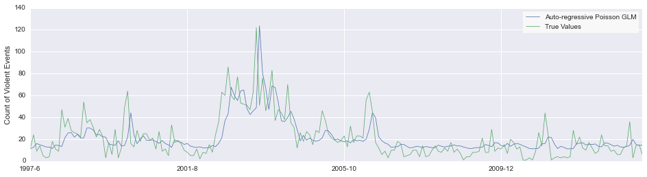
$$\begin{aligned} p(k | \mu_t) &= \frac{\mu_t^k}{k!}e^{-\mu_t} \\ p(k | \mathbf{X}_{t, \Lambda}, \beta) &= \frac{\log(\mathbf{X}_{t, \Lambda}'\beta)^k}{k!}e^{-\log(\mathbf{X}_{t, \Lambda}'\beta)} \end{aligned}$$

We can fit this model by using Fisher scoring to calculate $\beta_\mathrm{MLE}$, the coefficients of the model. Figure 7 shows this model as compared to actual rates of conflict incidence.

Putting together the spatial and temporal

We can now use our draws over space and time to generate a simulation of future conflicts in Uganda. These simulated scenarios will serve as the basis of our aid delivery optimization. The combination of modeling conflict events in space and time along with optimizing aid delivery could prove helpful to organizations such as the Red Cross in ordering supplies, allocating staff and volunteers, and developing infrastructure.